The expectation is not a sufficient measure for describing a distribution.

It is possible for two distributions with exactly the same expectation to have completely different statistical characteristics. We will illustrate this through an example. We will consider the following two distributions:

• Distribution A
  

  The Value	The Probability
  2	0.3
  3	0.25
  5	0.25
  7	0.2
  Total	1

• Distribution B
  

  The Value	The Probability
  0	0.25
  1	0.25
  7	0.25
  8	0.25
  Total	1

If, however, we insist on realistic examples, we can imagine two spinning wheels:

• One spinning wheel has the numbers 2, 3, 5, and 7 marked on it. Again, this spinning wheel is not balanced, meaning that certain numbers are more likely to appear than others. This spinning wheel corresponds to Distribution A.
• The second spinning wheel has the numbers 0, 1, 7, and 8 marked on it. Also, this spinning wheel is not balanced such that certain numbers are more likely to appear than others.This spinning wheel corresponds to Distribution B.

We will calculate the expectation of these two distributions:

Distribution A: (0.3 x 2) + (0.25 x 3) + (0.25 x 5) + (0.2 x 7) = 4

Distribution B: (0.25 x 0) + (0.25 x 1) + (0.25 x 7) + (0.25 x 8) = 4

The expectation of the distributions is identical: 4. But are these two distributions in fact identical?

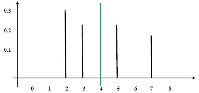
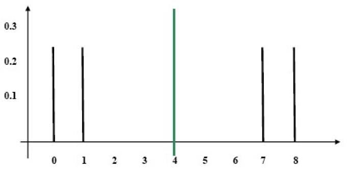
We will examine a stick diagram displaying the distributions (the dotted line denotes the expectation):

Distribution A

Diagram

Distribution B

Diagram

It is easy to see that Distribution B is more widely dispersed relative to the expectation than Distribution A. We will therefore use a measure of dispersal. A measure of the dispersal is a number that in effect expresses an estimate of the deviation from the expectation.

For mathematical reasons, however, our calculation is a little more complex, and includes squaring and taking the square root. The measure of the dispersal reflects the standard deviation or StDev. The method of calculating the StDev in the case of a probability is identical to the method for calculating the standard deviation of a sample.

We will add a third column, which we fill with the expectation, and a fourth column, in which we write the deviation from the expectation (the result of subtracting the expectation from the value).

The fifth column indicates the square of the deviation:

We will now calculate the expectation of the square of the deviation.

We multiply column 2 by column 5 and add: (0.3 x 4) + (0.25 x 1) + (0.25 x 1) + (0.2 x 9) = 3.5

The standard deviation reflects the square root of the result we previously obtained: (3.5)=1.87

In the same manner, we will calculate the StDev of Distribution B:

(0.25 x 16) + (0.25 x 9) + (0.25 x 9) + (0.25 x 16) = 12.5

The square root of 12.5 is 3.54.

As we expected, the StDev of Distribution B is greater than that of Distribution A.

Thus, Distribution B is more widely dispersed than Distribution A.