Why the Centrality Measures are Insufficient to Describe a Distribution?
We will consider the three data samples as lists of values; we can assume that they are students’ grades, for example:
Sample A: 7, 7, 7, 7, 7, 7, 7
Sample B: 10, 10, 7, 7, 7, 4, 4
Sample C: 8, 7, 7, 7, 7, 7, 6
These three samples have the same mode (7), the same median (7), and the same average (7). What then is the difference between these samples? It is easy to see that they do not have identical characteristics. The difference is in the way that they are dispersed.
Sample A is not dispersed at all, and it is concentrated upon a single point.
Sample B is the most dispersed of the three samples. It has values that are distant from the midpoint, and these values appear in significant numbers in the sample.
Sample C has moderate dispersal, i.e., the values are focused around the midpoint.
We will look at Additional Examples:
Samples with different midpoints are possible, but only if they have identical levels of dispersal. We will demonstrate this by using continuous variables:
We will conduct a sample of the heights (in centimeters) of residents in a certain city. 100 people were sampled, and the following results were obtained:
| The Values (Height) | The Frequency | The Relative Frequency | The Width of the Division | The Density |
| 140-150 | 10 | 10% | 10 | 1 |
| 150-160 | 20 | 20% | 10 | 2 |
| 160-170 | 40 | 40% | 10 | 4 |
| 170-180 | 20 | 20% | 10 | 2 |
| 180-190 | 10 | 10% | 10 | 1 |
| Total | 100 | 100% |
In another city, we will conduct a sample of the weights (in kilograms) of the residents. The number in the sample group was 500. The following illustrates the frequency table:
| The Values (Weight) | The Frequency | The Relative Frequency | The Width of the Division | The Density |
| 50-60 | 50 | 10% | 10 | 1 |
| 60-70 | 100 | 20% | 10 | 2 |
| 70-80 | 200 | 40% | 10 | 4 |
| 80-90 | 100 | 20% | 10 | 2 |
| 90-100 | 50 | 10% | 10 | 1 |
| Total | 500 | 100% |
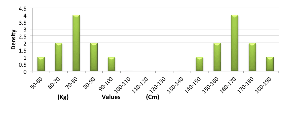
We will examine the histograms of the two samples:
The histogram of heights and weights:
Histogram

It is easy to see that the dispersal is identical, but the values around which the samples have been dispersed are different: 165 in the sample of heights, and 75 in the sample of weights.


